BUSINESS DATA SCIENCEの続き。

データなどは作者のgitにある。

Business Data Science: Combining Machine Learning and Economics to Optimize, Automate, and Accelerate Business Decisions

作者:Taddy, Matt
発売日: 2019/08/21
メディア: ハードカバー

最近「ビジネスデータサイエンスの教科書」という邦題で日本語版も出たみたいです

ビジネスデータサイエンスの教科書

作者:マット・タディ
発売日: 2020/07/22
メディア: 単行本

この章はなにか

分類問題について。

①は以下

knknkn.hatenablog.com

この節はなにか

多値分類について。

Multinomial Logistic Regression

前節までは0/1の2値(binary)分類をbinary logistic regressionでおこなったが、今回は多値(Multinomial)分類をおこなうため multinomial logistic regressionを考える。

このとき、例えば分類k = (1,2,3)の全3分類があった上で、 $y_i = 2$ が正解ラベルのとき、 $y_i = (0, 1, 0)$ のように自クラスを1、それ以外を0として表現をしなおすことで、前節のbinary logistic regressionと同様におこなうことができる。ただし、このとき分類毎の各変数への係数 $B = (\beta_1,\beta_2,...\beta_k)$ も推定する必要がある。

また、全分類を考慮した1となる確率は以下となる。

$p(y_i = 1 | x) = \frac{e^{x' \beta_i}}{\sum_{k=1}^{K} e^{x' \beta_k}}$

そのため、各変数への係数 $B = (\beta_1,\beta_2,...\beta_k)$ を全て用いたdevianceは以下となる。

$-2\sum_i \sum_k y_{ik} log(p_{ik}(x'_i B)) = -2 \sum_{i=1}^n (\sum_{k=1}^K y_{ik}\, x'_i \beta_k - m_i\, log(e^{x'_i \beta_k}))$

なお、 $m_i$ は $\sum_k y_{ik}$ のことを指し、これは正解となる分類の数を表す。k=2のみが正解ラベルのとき $m_i = 1$ となり、 k = 2,3の2つが正解のとき $m_i = 2$ となる。複数が正解はテキストマイニングなどでは使う概念。

このdevianceは各変数への係数Bを用いているので、全分類を考慮してdivianceを最小にするようにする必要がある。ペナルティ項を付与して最小化すると以下を考えることになる。

$argmin(- \frac{2}{n} \sum_i ^n y_{ik} log(p_{ik}(x'_i B) + λ \sum_k \sum_j |\beta_{kj}|)$

このとき式からわかるようにλは各分類に対して共通のλを用いる。

実データ

前回使ったガラスについてのデータ。

github.com

各ガラスタイプ毎にlassoでCVすると以下のようになる。

## A lasso penalized multinomial regression model
## running and plotting with glmnet
library(glmnet)
## we'll consider all of the content variables, interacted with RI
## You could also look at all interactions; you get diff model but similar performance OOS
xfgl <- sparse.model.matrix(type~.*RI, data=fgl)[,-1]
gtype <- fgl$type

glassfit <- cv.glmnet(xfgl, gtype, family="multinomial")
plot(glassfit) # CV error; across top avg # nonzero across classes
## plot the 6 sets of coefficient paths for each response class
par(mfrow=c(2,3), mai=c(.6,.6,.4,.4)) ## note we can use xvar="lambda" to plot against log lambda
plot(glassfit$glm, xvar="lambda")

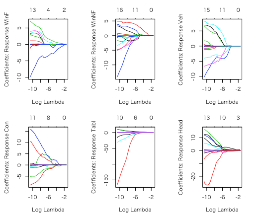
f:id:chito_ng:20200324200345p:plain

このとき、各ガラスタイプによって挙動が異なっているが、モデルは全結果のdevianceであるmultinomial deviance(のペナルティ項付き)を最小にする共通のλを用いている。

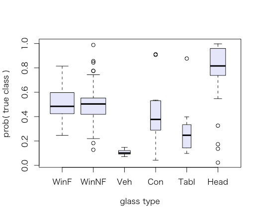
$multinomial deviance = -2 \sum_{i} \sum_{k} y_{ik} log(p_{ik})$

また、このモデルでの各ガラスタイプに対して、各ガラスタイプと予測している確率は以下のようになる。

### fit plots: plot p_yi distribution for each true yi
# use predict to get in-sample probabilities
probfgl <- predict(glassfit, xfgl, type="response")
# for some reason glmnet gives back predictions as an nxKx1 array. 
# use drop() to make it an nxK matrix
probfgl <- drop(probfgl)
# get the probs for what actually happened
# note use of a matrix to index a matrix! 
# gives back the [i,j] entry of probfgl for each row of index matrix 
# so, here, that's the probability of true class for each observation
n <- nrow(xfgl)
trueclassprobs <- probfgl[cbind(1:n, gtype)] 
## plot true probs, with varwidth to have the box widths proportional to response proportion.
plot(trueclassprobs ~ gtype, col="lavender", varwidth=TRUE,
     xlab="glass type", ylab="prob( true class )")

f:id:chito_ng:20200324201211p:plain

Distributed Multinomial Regression

multinomial logistic regressionを用いた場合、求めたい分類の係数以外の全ての分類係数を考慮して1式で表しているので計算に時間がかかる。

multinomial logistic regressionで前提としている多項分布(Multinomial Distribution)の係数は、ある条件下でのポアソン分布に近似できることが知られている。

qiita.com

そのため、ポアソン分布を用いて $\beta_k$ をk毎にkの係数のみを考慮して各分類ごとに個別の式で求めることができる。

$y_{ik} ~ Poisson(exp(x'_i \beta_k))$

そのため、 $\beta_k$ の推定は以下となる。

$deviance(\beta_k) ∝ \sum_{i=1}^n exp(x'_i β_k) - y_i(x'_i β_k)$

よって、ペナルティ項を含めると以下を最小にする $\beta_k$ を推定する。

$argmin( \sum_{i=1}^n exp(x'_i β_k) - y_i(x'_i β_k) + λ_k \sum_j | \beta_{kj}|)$

となる。

前節のときと比較すると、k毎にλも個別で求めているのでより緻密な推定ができる。

また、個別で求めていることから並列計算が可能になることで速度が向上する。

####  Moving to distrom
library(distrom) # library(parallel)
detectCores()
# 4
cl = makeCluster(4)
cl
# socket cluster with 4 nodes on host ‘localhost’

実データ

先ほどと同様にガラスデータ。

dmr を用いると、多値分類において前述のポアソン分布を用いた並列計算をおこなった結果をgamlr と同様のオブジェクトで返す(なお、先程はgamlrではなくgmlnetを使っているが同様のオブジェクトを返す)。

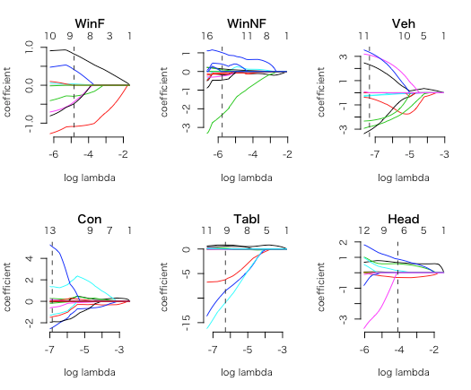
glassdmr <- dmr(cl, xfgl, gtype, verb=TRUE)
names(glassdmr)
#  "WinF"  "WinNF" "Veh"   "Con"   "Tabl"  "Head" 

glassdmr[["WinF"]]
# poisson gamlr with 17 inputs and 100 segments.

gamlr (gmlnet)ではkで共通のλを使っているが今回は前述のようにk毎で別のλが使われていることがわかる。

## plot a set of paths
par(mfrow=c(2,3))
for(k in names(glassdmr)) plot(glassdmr[[k]], main=k)  
## and grab the AICc selected coefficients
Bdmr <- coef(glassdmr)
round(Bdmr,1)
# 18 x 6 sparse Matrix of class "dmrcoef"
# WinF WinNF   Veh   Con  Tabl  Head
# intercept -28.4  13.4 169.4 118.2 -12.1 -22.2
# RI          .     .     .     .     .     .  
# Na         -0.3  -0.2  -0.3  -2.5   0.6   0.6
# Mg          0.8   .     2.3  -1.5   .    -0.3
# Al         -1.1   0.4  -0.4   1.4   0.8   0.9
# Si          0.4  -0.1  -2.8  -1.3   .     0.1
# K           .     .    -3.1   .    -8.5   .  
# Ca          .    -0.5   3.3   0.3   0.2   .  
# Ba          .    -2.3   .     .    -6.2   0.7
# Fe         -0.5   1.0  -2.3   5.1 -10.9   .  
# RI:Na       .     .     .     0.2   .     .  
# RI:Mg       0.0  -0.1   .    -0.1  -0.1   .  
# RI:Al       .    -0.1   .     .     .     .  
# RI:Si       .     0.0   .     .     .     .  
# RI:K        .     0.1   .     .     .     .  
# RI:Ca       .     .    -0.2  -0.2   0.0   .  
# RI:Ba       .     0.1   .    -0.6   .     .  
# RI:Fe      -0.4  -0.2   3.1  -1.9   .

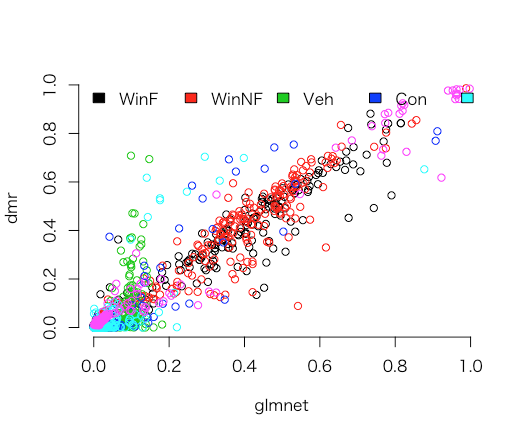
f:id:chito_ng:20200325100114p:plain

今回のように、小標本数(n=214)のときはdmrとglmnet(gamlr)で予測に大きな違いは起きない(下図は真のラベルに対する確率をdmrとgamlr毎に出している)が、大標本ではdmrの方が良い推定となることが多い。これは、k毎にλを変えていることが原因となる。

## it's because of the variable lambda (diff lambda accross classes),
## and because we're using AICc rather than CV selection.
## the predictions are roughly close though.
# note you can call predict on glassdmr or Bdmr and get the
# same answer (latter's a bit faster for big datasets)
pdmr <- predict(Bdmr,xfgl,type="response")
plot(probfgl,pdmr,col=rep(1:6,each=n),xlab="glmnet",ylab="dmr",bty="n")
legend("topleft", fill=1:6, legend=levels(gtype), bty="n",h=TRUE)