LightGBMを試してみる。　　 LightGBMはBoosted treesアルゴリズムを扱うためのフレームワークで、XGBoostよりも高速らしい。

XGBoostやLightGBMに共通する理論のGradient Boosting Decision Treeとは、弱学習器としてDecision Treeを用いたBoostiongアンサンブル学習のことを指す。

アンサンブル学習として、Boostingではなく、Bagging（の類似）だとランダムフォレストになるのかな？

knknkn.hatenablog.com

www.codexa.net

とりあえず使ってみるということで、理論などは置いとく。ちなみに下記がわかりやすかった。

また、XGBoostの理論だが下記がわかりやすかった。XGBoostとLightGBMの違いは、決定木で学習するときにXGBoostではpre-sortedベース、LightGBMではhistogram based algorithmsを用いるという差があるがそれ以外の基本的なところは同じなので理解の参考にした。

qiita.com

kefism.hatenablog.com

データ

irisは簡単すぎるしなぁ、ということでtitanicを使用する。
なお、今回は以下を参考にしている(というか、トレースしただけ)。

Applying LightGBM to Titanic dataset | Kaggle

トレース

データ読み込み

# https://www.kaggle.com/shep312/applying-lightgbm-to-titanic-dataset

import pandas as pd
import numpy as np
import matplotlib.pyplot as plt
import lightgbm as lgbm # lgbとしている記載が多いが元ソースに合わせる
from sklearn.model_selection import train_test_split
from sklearn.preprocessing import LabelEncoder
from sklearn.metrics import accuracy_score, recall_score, precision_score, f1_score
%matplotlib inline

train_df = pd.read_csv('./input/train.csv')
test_df = pd.read_csv('./input/test.csv')
train_df.info()

<class 'pandas.core.frame.DataFrame'>
RangeIndex: 891 entries, 0 to 890
Data columns (total 12 columns):
PassengerId    891 non-null int64
Survived       891 non-null int64
Pclass         891 non-null int64
Name           891 non-null object
Sex            891 non-null object
Age            714 non-null float64
SibSp          891 non-null int64
Parch          891 non-null int64
Ticket         891 non-null object
Fare           891 non-null float64
Cabin          204 non-null object
Embarked       889 non-null object
dtypes: float64(2), int64(5), object(5)
memory usage: 83.6+ KB

Feature engineering

いくつかFeatureを足す
カテゴリ変数Embarked, Sexを数値にエンコードする => LGBMではint, float, booleanしか渡すことができないので、カテゴリ変数(object)を整数値（int)として渡す必要があるため。
利用が難しそうなFeatureを落とす

また、カテゴリ変数のエンコードはsklearn.preprocessing.LabelEncoderを用いる。

scikit-learn.org

# Not sure passenger ID is useful as a feature, but need to save it from the test set for the submission
test_passenger_ids = test_df.pop('PassengerId')
train_df.drop(['PassengerId'], axis=1, inplace=True)

# 'Embarked' is stored as letters, so fit a label encoder to the train set to use in the loop
embarked_encoder = LabelEncoder()
embarked_encoder.fit(train_df['Embarked'].fillna('Null'))

# Dataframes to work on
df_list = [train_df, test_df]

for df in df_list:    
    
    # Record anyone travelling alone
    df['Alone'] = (df['SibSp'] == 0) & (df['Parch'] == 0)
    
    # Transform 'Embarked'
    df['Embarked'].fillna('Null', inplace=True)
    df['Embarked'] = embarked_encoder.transform(df['Embarked'])
    
    # Transform 'Sex'
    df.loc[df['Sex'] == 'female','Sex'] = 0
    df.loc[df['Sex'] == 'male','Sex'] = 1
    df['Sex'] = df['Sex'].astype('int8')
    
    # Drop features that seem unusable. Save passenger ids if test
    df.drop(['Name', 'Ticket', 'Cabin'], axis=1, inplace=True)

Prep the training set for learning

トレーニングデータを準備する。

Hold-Out法で訓練データとテストデータを2:8で分ける。
lgbmオブジェクトという形で作成する。

# Separate the label
y = train_df.pop('Survived')

# Take a hold out set randomly
X_train, X_test, y_train, y_test = train_test_split(train_df, y, test_size=0.2, random_state=42)

# Create an LGBM dataset for training
categorical_features = ['Alone', 'Sex', 'Pclass', 'Embarked']
train_data = lgbm.Dataset(data=X_train, label=y_train, categorical_feature=categorical_features, free_raw_data=False)

# Create an LGBM dataset from the test
test_data = lgbm.Dataset(data=X_test, label=y_test, categorical_feature=categorical_features, free_raw_data=False)

# Finally, create a dataset for the FULL training data to give us maximum amount of data to train on after 
# performance has been calibrate
final_train_set = lgbm.Dataset(data=train_df, label=y, 
                               categorical_feature=categorical_features, free_raw_data=False)

Define hyperparameters for LGBM

ハイパーパラメータを決める。ハイパーパラメータは大まかにいうと3種類に分かれている。

Tree-Specific Parameters: ツリー固有パラメータ：ツリーの形状や動作などを規定するパラメータ
Boosting Parameters: ブースティングパラメータ：勾配動作などを規定するパラメータ
Miscellaneous Parameters: 他パラメータ

今回は生死(0/1)の二値（バイナリ）分類なのでapplicationをbinaryにする。決めるハイパーパラメータの内容は以下参考。

lightgbm.readthedocs.io

ドキュメント以外だとこのあたり？

www.analyticsvidhya.com

qiita.com

rautaku.hatenablog.com

lgbm_params = {
    'boosting': 'dart',          # dart (drop out trees) often performs better
    'application': 'binary',     # Binary classification
    'learning_rate': 0.05,       # Learning rate, controls size of a gradient descent step
    'min_data_in_leaf': 20,      # Data set is quite small so reduce this a bit
    'feature_fraction': 0.7,     # Proportion of features in each boost, controls overfitting
    'num_leaves': 41,            # Controls size of tree since LGBM uses leaf wise splits
    'metric': 'binary_logloss',  # Area under ROC curve as the evaulation metric
    'drop_rate': 0.15
              }

Train the model

ホールド・アウト法で検証して、パフォーマンスを評価。また、early stopをおこない適当なところで学習をストップ。

結果はevaluation_resultsに格納。また、best_iterationを用いて最も良いスコアのときの回数をoptimum_boost_roundsに格納。

evaluation_results = {}
clf = lgbm.train(train_set=train_data,
                 params=lgbm_params,
                 valid_sets=[train_data, test_data], 
                 valid_names=['Train', 'Test'],
                 evals_result=evaluation_results,
                 num_boost_round=500,
                 early_stopping_rounds=100,
                 verbose_eval=20
                )
optimum_boost_rounds = clf.best_iteration

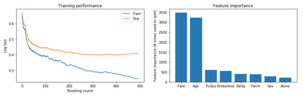
Visualise training performance

パフォーマンスを可視化

fig, axs = plt.subplots(1, 2, figsize=[15, 4])

# Plot the log loss during training
axs[0].plot(evaluation_results['Train']['binary_logloss'], label='Train')
axs[0].plot(evaluation_results['Test']['binary_logloss'], label='Test')
axs[0].set_ylabel('Log loss')
axs[0].set_xlabel('Boosting round')
axs[0].set_title('Training performance')
axs[0].legend()

# Plot feature importance
importances = pd.DataFrame({'features': clf.feature_name(), 
                            'importance': clf.feature_importance()}).sort_values('importance', ascending=False)
axs[1].bar(x=np.arange(len(importances)), height=importances['importance'])
axs[1].set_xticks(np.arange(len(importances)))
axs[1].set_xticklabels(importances['features'])
axs[1].set_ylabel('Feature importance (# times used to split)')
axs[1].set_title('Feature importance')

plt.show()

f:id:chito_ng:20190128091525p:plain

Examine model performance

精度などを見る。ドキュメント的には以下のClassification metrics。

scikit-learn.org

Accuracy score: 正解率。1のものは1として分類(予測)し、0のものは0として分類した割合
Precision score: 精度。1に分類したものが実際に1だった割合
Recall score: 検出率。1のものを1として分類(予測)した割合
F1 score: PrecisionとRecallを複合した0~1のスコア。数字が大きいほど良い評価。

preds = np.round(clf.predict(X_test))
print('Accuracy score = \t {}'.format(accuracy_score(y_test, preds)))
print('Precision score = \t {}'.format(precision_score(y_test, preds)))
print('Recall score =   \t {}'.format(recall_score(y_test, preds)))
print('F1 score =      \t {}'.format(f1_score(y_test, preds)))

Accuracy score =      0.8379888268156425
Precision score =    0.8260869565217391
Recall score =       0.7702702702702703
F1 score =           0.7972027972027972

Make predictions on the test set

num_boost_roundを最適な回数(optimum_boost_rounds)にして再度分類をする。

clf_final = lgbm.train(train_set=final_train_set,
                      params=lgbm_params,
                      num_boost_round=optimum_boost_rounds,
                      verbose_eval=0
                      )

y_pred = np.round(clf_final.predict(test_df)).astype(int)

output_df = pd.DataFrame({'PassengerId': test_passenger_ids, 'Survived': y_pred})

まずは蝋の翼から。

学んだことを書きながら確認・整理するためのメモブログ。こういうことなのかな？といったことをふわっと書いたりしていますが、理解が浅いゆえに的はずれなことも多々あると思うのでツッコミ歓迎

LightGBMを試す

データ