特徴量作成を楽にするライブラリいくつかまとめて試す① featuretools
この記事はなにか
機械学習の特徴量を作るときに色々とめんどくさい部分を楽にできるライブラリの紹介。
具体的には以下を紹介する、
- featuretools
- xfeat
①では既存特徴量を四則演算したり集約したり、date型の年部分のみ取り出すなど、既存特徴量をもとに色々加工するのに便利なライブラリfeaturetoolsについて。
機械学習において「とりあえず既存特徴量を四則演算/集約でいじくりまわす」だけでもそれなりに精度が上がる*1ことから、それらを脳死で作成しまくることはそれなりに有効だが、コードを書くのが面倒なことも多い。これを楽にできるのが featuretools
何を書かないか
基本的な使い方などをメモ代わりに試すだけなので、取り扱いの詳細は公式ドキュメントか適宜貼るリンクを読んでくれというスタイルで書く。
featuretools
内部的に、複数データフレームの関係性込みでER図っぽい感じでデータを持つオブジェクトを作成しその情報をもとに指定した基礎集計をデータ型に応じていい感じにしてくれる。なお、型に応じた処理をしてくれる性質上pandasよりも型の種類は多いし、基礎集計もSQLの関数レベルであればデータ処理に使うものはだいたいある。
複数テーブルのあるデモデータで試す
いったん通常のやり方として、featuretoolsにあるデモデータで例示する。
なお、コードは以下の記事を参照した
import featuretools as ft
data = ft.demo.load_mock_customer()
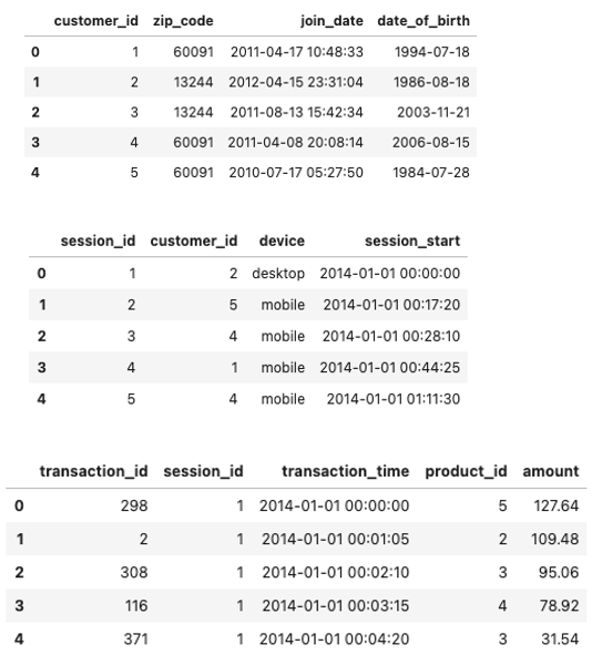
display(data['customers'].head(),
data['sessions'].head(),
data['transactions'].head())
流れとしては、
1. EntitysetというER的なデータとデータ関係が入ったオブジェクトを作成
# EntitySetインスタンスの作成
es = ft.EntitySet(id='demo') # idはEntitySet名

# Entityとしてデータフレームを登録
es.entity_from_dataframe(entity_id='cust', # entity名
                         dataframe=data['customers'], # 登録するDF
                         index='customer_id') # ユニークとなるためのindex

es.entity_from_dataframe(entity_id='session',
                         dataframe=data['sessions'],
                         index='session_id',
                         time_index='session_start') # 時系列で認識させたい場合

es.entity_from_dataframe(entity_id='trans',
                         dataframe=data['transactions'],
                         index='transaction_id',
                         time_index='transaction_time')
その結果esは以下のような出力となる。
Entityset: demo
  Entities:
    cust [Rows: 5, Columns: 4]
    session [Rows: 35, Columns: 4]
    trans [Rows: 500, Columns: 5]
  Relationships:
    No relationships
見たままですが、demoという名前のEntitySetで、Entityとしてはcust, session, transの3つをもち、それぞれのshapeも書いてます。また、No relationshipsとあるように現段階ではEntityのひも付きはないので紐付けます
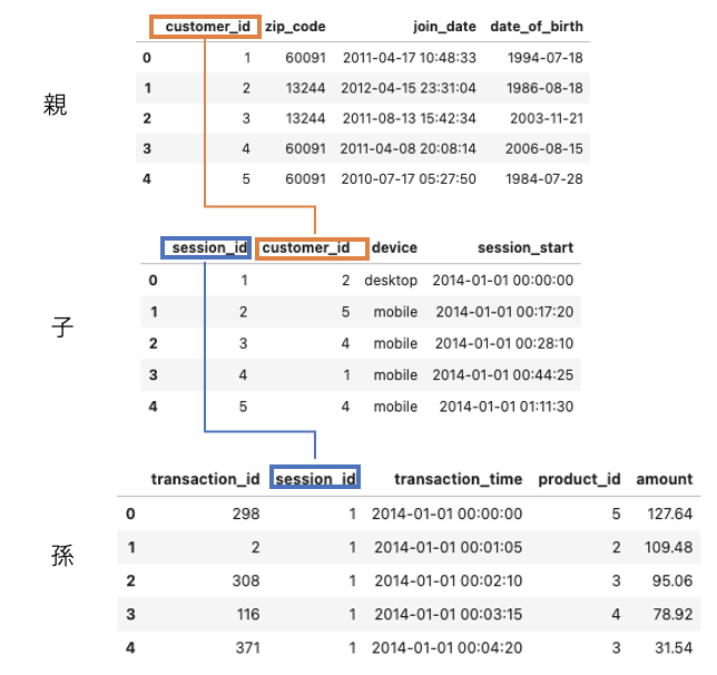
# relationの定義
# Relationship(親, 子)とする
r_cust_session = ft.Relationship(es['cust']['customer_id'], es['session']['customer_id'])
r_session_trans = ft.Relationship(es['session']['session_id'], es['trans']['session_id'])

# 紐付け
es.add_relationships(relationships=[r_cust_session,r_session_trans])
esをみると紐付けが完了してる
Entityset: demo
  Entities:
    cust [Rows: 5, Columns: 4]
    session [Rows: 35, Columns: 4]
    trans [Rows: 500, Columns: 5]
  Relationships:
    session.customer_id -> cust.customer_id
    trans.session_id -> session.session_id
ちなみに、Entityの情報(列や型、shape)をみたり、DFで呼び戻したりは以下のようにしてできる
# Entityの情報を表示
es['cust']

# =>
# Entity: cust
#  Variables:
#    customer_id (dtype: index)
#   zip_code (dtype: categorical)
#  join_date (dtype: datetime)
#    date_of_birth (dtype: datetime)
#  Shape:
#    (Rows: 5, Columns: 4)


# dfで戻す
df_cust = es['cust'].df
集計/変換処理をする
本題。型や関係性に応じて集計や変換をする。Entityを横断的に集計処理をすることをDeep Feature Synthesis(DFS)というそうな。
DFS処理をするメソッドdfsを使う。返り値は集計結果のDFとそのDFの特徴量定義情報
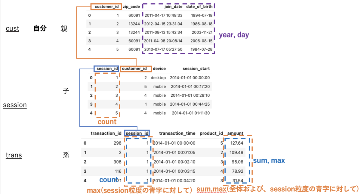
# 適用したい集約関数
list_agg = ['sum','max','count']

# 適用したい変換関数
list_trans = ['year','day']

# run dfs
df_feature, features_defs = ft.dfs(entityset=es, # 適用先entityset名
                                     target_entity='cust', # 適用先entity
                                     agg_primitives=list_agg, # 適用集約関数
                                     trans_primitives =list_trans, #適用変換関数
                                     max_depth=1 #適用の深さ
                                   )
# head
df_feature.head()
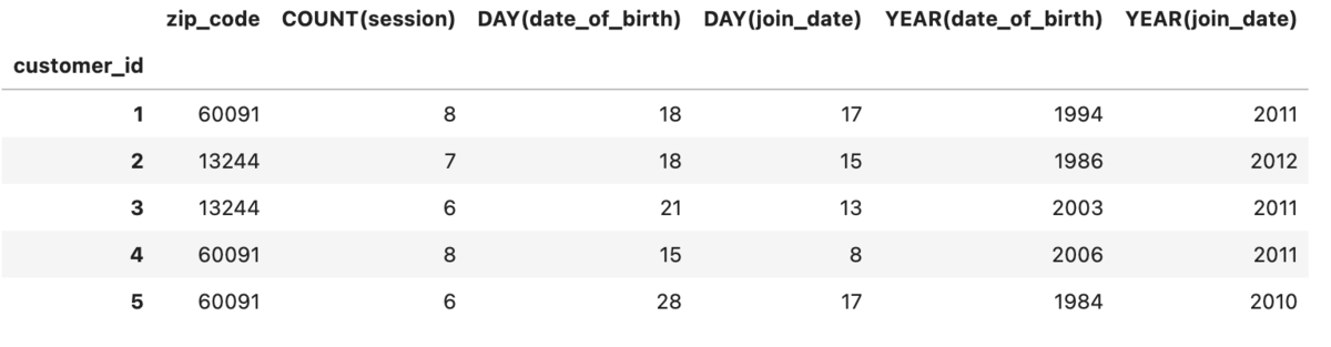
このとき、target_entityを起点にagg_primitivesはmax_depthの深さまで、trans_primitivesは自身に適用される。
今回target_entityは最上部のcustとなので、agg_primitivesのsum,max,countは子であるsessionテーブルのうちこれらが適用可能な列に適用され(数値がないためsum,maxは不使用で、sessionテーブルの行数countのみ適用される)、trans_primitivesのyear,dayは自身の適用可能な列に適用される。
次にmax_depth=2を考える。
# 適用したい集約関数
list_agg = ['sum','max','count']

# 適用したい変換関数
list_trans = ['year','day']

# run dfs
df_feature, features_defs = ft.dfs(entityset=es, # 適用先entityset名
                                     target_entity='cust', # 適用先entity
                                     agg_primitives=list_agg, # 適用集約関数
                                     trans_primitives =list_trans, #適用変換関数
                                     max_depth=2 #適用の深さ
                                   )
features_defsは以下。
features_defs
=>
[<Feature: zip_code>,
 <Feature: COUNT(session)>,
 <Feature: COUNT(trans)>,
 <Feature: MAX(trans.amount)>,
 <Feature: SUM(trans.amount)>,
 <Feature: DAY(date_of_birth)>,
 <Feature: DAY(join_date)>,
 <Feature: YEAR(date_of_birth)>,
 <Feature: YEAR(join_date)>,
 <Feature: MAX(session.COUNT(trans))>,
 <Feature: MAX(session.SUM(trans.amount))>,
 <Feature: SUM(session.MAX(trans.amount))>]
trans_primitivesは自身のみのままだが、agg_primitivesの適用の深さが変わっている。
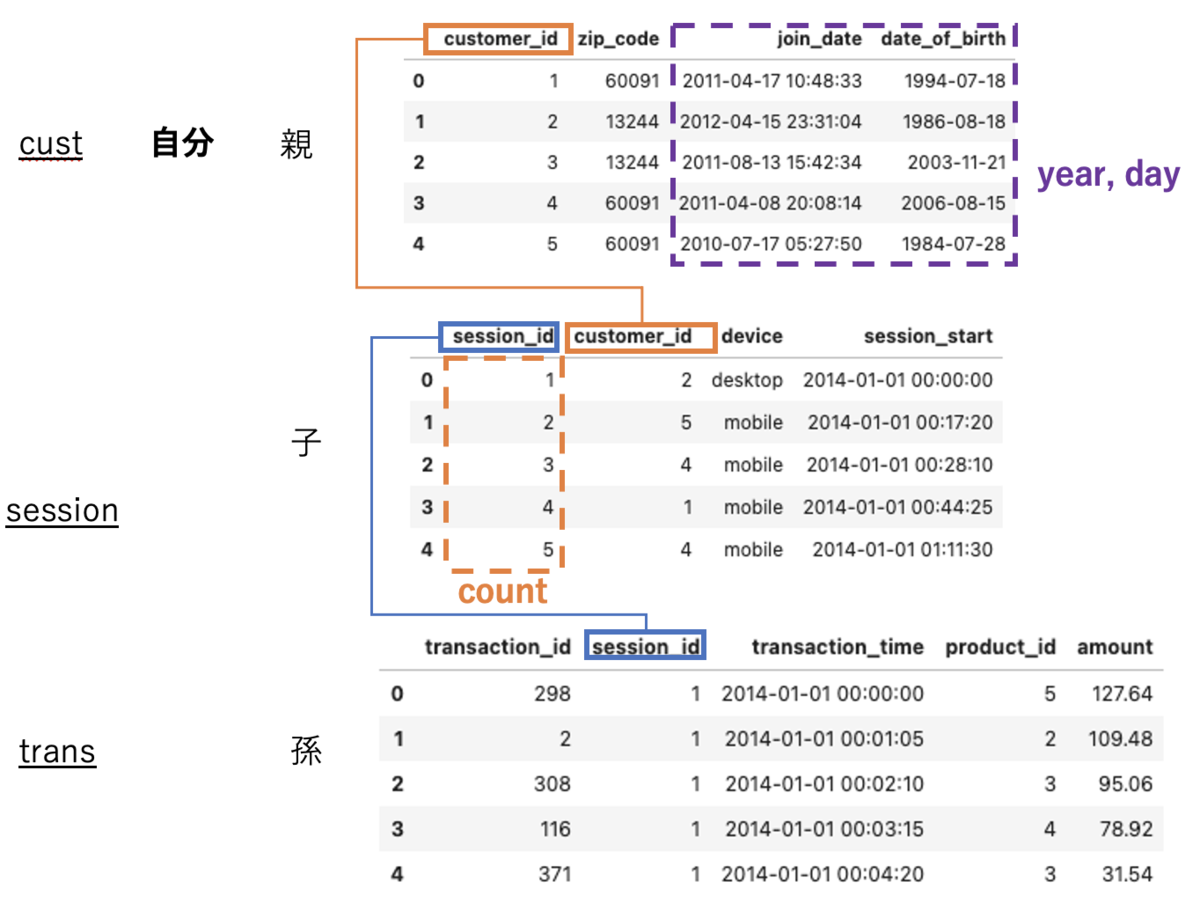
1. 深さ1(子)に対して自身の粒度で集計
2. 深さ2(孫)に対して自身の粒度で集計
3. 深さ1(子)粒度で深さ2(孫)を集計し、その値に対して自身の集計を更にかける(例: MAX(session.SUM(trans.amount))は孫のtrans.amountを子のsession(session_id)粒度でSUMをしてその後自身のcust(custmar_id)の粒度で集計している。
なお、primitives適用をした列以外の列は自身が持つ列以外は残らない模様(正確には、自身より上のレイヤーがある場合はmax_depthによっては紐づく)。
次に、target_entityを子にして同様のことをする。
まずは次にmax_depth=1
# run dfs
df_feature, features_defs = ft.dfs(entityset=es, # 適用先entityset名
                                     target_entity='session', # 適用先entity
                                     agg_primitives=list_agg, # 適用集約関数
                                     trans_primitives =list_trans, #適用変換関数
                                     max_depth=1 #適用の深さ
                                   )
# head
df_feature.head()
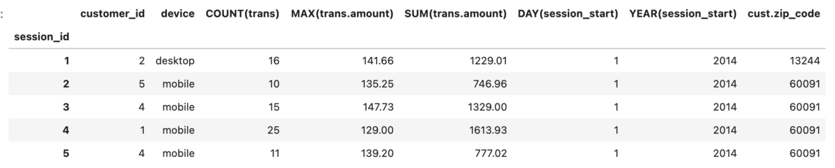
このとき、前回同様にtarget_entityであるsessionを起点にagg_primitivesはmax_depthの深さまで、trans_primitivesは自身に適用される。
注意する点としては
- max_depthは前後に効くので親と子ともに紐づく
- 自分より(max_depth内の)上位のテーブルの特徴量を取ってくる。
2.はcust.zip_codeが紐付いていることからそう判断しましたが、join_date date_of_birthを取ってこないのはなんでや。。。型によって取ってくるものと取ってこないものがあるのかも?
次にmax_depth=2
df_feature, features_defs = ft.dfs(entityset=es, # 適用先entityset名
                                     target_entity='session', # 適用先entity
                                     agg_primitives=list_agg, # 適用集約関数
                                     trans_primitives =list_trans, #適用変換関数
                                     max_depth=2 #適用の深さ
                                   )
features_defs

<Feature: customer_id>,
 <Feature: device>,
 <Feature: COUNT(trans)>,
 <Feature: MAX(trans.amount)>,
 <Feature: MIN(trans.amount)>,
 <Feature: SUM(trans.amount)>,
 <Feature: DAY(session_start)>,
 <Feature: MONTH(session_start)>,
 <Feature: YEAR(session_start)>,
 <Feature: cust.zip_code>,
 <Feature: cust.COUNT(session)>,
 <Feature: cust.COUNT(trans)>,
 <Feature: cust.MAX(trans.amount)>,
 <Feature: cust.MIN(trans.amount)>,
 <Feature: cust.SUM(trans.amount)>,
 <Feature: cust.DAY(date_of_birth)>,
 <Feature: cust.DAY(join_date)>,
 <Feature: cust.MONTH(date_of_birth)>,
 <Feature: cust.MONTH(join_date)>,
 <Feature: cust.YEAR(date_of_birth)>,
 <Feature: cust.YEAR(join_date)>]
<Feature: cust.COUNT(session)>以下が差分。
正直わっかんねーなーってとこはあるんですが、自分より上に対してもtrans_primitives agg_primitivesが適用されている(厳密には、上に対してtrans_primitivesが適用&上の粒度でそれより下に対してagg_primitivesで集約される?)。そこから考えるに、
trans_primitivesは自身か自身より上に適用。ただし自身以上の場合は1遅延がある(深さ2なら、2-1=1上まで)?agg_primitivesは自身より下か自身より上に適用。ただし自身以上の場合は1遅延がある(深さ2なら、2-1=1上まで)?
といったところでしょうか?まぁ正直挙動がわかりづらいんですが、基本的に最上位層をtarget_entityにして分析することがほとんどだと思うのでそこまで気にしなくていいのかも。
1テーブルのデータで試す
ボストンの住宅価格情報データセットBoston Housingを使う。
詳細は以下
import pandas as pd
import numpy as np

from sklearn.datasets import load_boston

boston = load_boston()

df_X = pd.DataFrame(boston.data, columns=boston.feature_names)
df_y = pd.DataFrame(boston.target, columns=['target'])

# 年齢を四捨五入したものを追加
df_X['AGE2'] = df_X['AGE'].round(-1)
こちらは特に複数テーブルがあるわけではないので、自らマスタデータのようなものを作る必要がある。
# EntitySetインスタンスの作成
es = ft.EntitySet(id='Boston') # idはEntitySet名

# Entityとしてデータフレームを登録
es.entity_from_dataframe(entity_id='features', # entity名
                         dataframe=df_X, # 登録するDF
                         index='index') # ユニークとなるためのindex
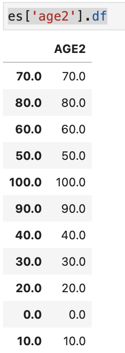
DFSをするにはrelationが必要だがこのままではrelationがないので、集約したい列のマスタテーブルのようなものをつくり紐付ける。これはnormalize_entityでできる。
es = es.normalize_entity(base_entity_id='features',
                         new_entity_id='age2',
                         index='AGE2',
                        )

# Entityset: Boston
#  Entities:
#    features [Rows: 506, Columns: 15]
#    age2 [Rows: 11, Columns: 1]
# Relationships:
#    features.AGE2 -> age2.AGE2
list_agg = ['sum','max','count']
list_trans = ['subtract_numeric', 'multiply_numeric'] # 減算/乗算の組み合わせ

# run dfs
df_feature, features_defs = ft.dfs(entityset=es, # 適用先entityset名
                                     target_entity='features', # 適用先entity
                                     agg_primitives=list_agg, # 適用集約関数
                                     trans_primitives =list_trans, #適用変換関数
                                     max_depth=2 #適用の深さ
                                   )
# 特徴量
features_defs
デモデータでは集計値に対して更に集計していたが、こちらでは変換したものに対しての集計がおこなわれている。
そのため、総じて言えばmax_depthを深くするとその手前の深さの処理(集約や変換)に対しても更に集約が走ると捉えれる。
[<Feature: CRIM>,
 <Feature: ZN>,
 <Feature: INDUS>,
 <Feature: CHAS>,
 <Feature: NOX>,
 <Feature: RM>,
 <Feature: AGE>,
 <Feature: DIS>,
 <Feature: RAD>,
 <Feature: TAX>,
 <Feature: PTRATIO>,
 <Feature: B>,
 <Feature: LSTAT>,
 <Feature: AGE2>,
 <Feature: AGE * B>,
 <Feature: AGE * CHAS>,
 <Feature: AGE * CRIM>,
 <Feature: AGE * DIS>,
 <Feature: AGE * INDUS>,
 <Feature: AGE * LSTAT>,
 <Feature: AGE * NOX>,
 <Feature: AGE * PTRATIO>,
 <Feature: AGE * RAD>,
 <Feature: AGE * RM>,
 <Feature: AGE * TAX>,
 <Feature: AGE * ZN>,
 <Feature: B * CHAS>,
 <Feature: B * CRIM>,
 <Feature: B * DIS>,
 <Feature: B * INDUS>,
 <Feature: B * LSTAT>,
 <Feature: B * NOX>,
 <Feature: B * PTRATIO>,
 <Feature: B * RAD>,
 <Feature: B * RM>,
 <Feature: B * TAX>,
 <Feature: B * ZN>,
 <Feature: CHAS * CRIM>,
 <Feature: CHAS * DIS>,
 <Feature: CHAS * INDUS>,
 <Feature: CHAS * LSTAT>,
 <Feature: CHAS * NOX>,
 <Feature: CHAS * PTRATIO>,
 <Feature: CHAS * RAD>,
 <Feature: CHAS * RM>,
 <Feature: CHAS * TAX>,
 <Feature: CHAS * ZN>,
 <Feature: CRIM * DIS>,
 <Feature: CRIM * INDUS>,
 <Feature: CRIM * LSTAT>,
 <Feature: CRIM * NOX>,
 <Feature: CRIM * PTRATIO>,
 <Feature: CRIM * RAD>,
 <Feature: CRIM * RM>,
 <Feature: CRIM * TAX>,
 <Feature: CRIM * ZN>,
 <Feature: DIS * INDUS>,
 <Feature: DIS * LSTAT>,
 <Feature: DIS * NOX>,
 <Feature: DIS * PTRATIO>,
 <Feature: DIS * RAD>,
 <Feature: DIS * RM>,
 <Feature: DIS * TAX>,
 <Feature: DIS * ZN>,
 <Feature: INDUS * LSTAT>,
 <Feature: INDUS * NOX>,
 <Feature: INDUS * PTRATIO>,
 <Feature: INDUS * RAD>,
 <Feature: INDUS * RM>,
 <Feature: INDUS * TAX>,
 <Feature: INDUS * ZN>,
 <Feature: LSTAT * NOX>,
 <Feature: LSTAT * PTRATIO>,
 <Feature: LSTAT * RAD>,
 <Feature: LSTAT * RM>,
 <Feature: LSTAT * TAX>,
 <Feature: LSTAT * ZN>,
 <Feature: NOX * PTRATIO>,
 <Feature: NOX * RAD>,
 <Feature: NOX * RM>,
 <Feature: NOX * TAX>,
 <Feature: NOX * ZN>,
 <Feature: PTRATIO * RAD>,
 <Feature: PTRATIO * RM>,
 <Feature: PTRATIO * TAX>,
 <Feature: PTRATIO * ZN>,
 <Feature: RAD * RM>,
 <Feature: RAD * TAX>,
 <Feature: RAD * ZN>,
 <Feature: RM * TAX>,
 <Feature: RM * ZN>,
 <Feature: TAX * ZN>,
 <Feature: AGE - B>,
 <Feature: AGE - CHAS>,
 <Feature: AGE - CRIM>,
 <Feature: AGE - DIS>,
 <Feature: AGE - INDUS>,
 <Feature: AGE - LSTAT>,
 <Feature: AGE - NOX>,
 <Feature: AGE - PTRATIO>,
 <Feature: AGE - RAD>,
 <Feature: AGE - RM>,
 <Feature: AGE - TAX>,
 <Feature: AGE - ZN>,
 <Feature: B - CHAS>,
 <Feature: B - CRIM>,
 <Feature: B - DIS>,
 <Feature: B - INDUS>,
 <Feature: B - LSTAT>,
 <Feature: B - NOX>,
 <Feature: B - PTRATIO>,
 <Feature: B - RAD>,
 <Feature: B - RM>,
 <Feature: B - TAX>,
 <Feature: B - ZN>,
 <Feature: CHAS - CRIM>,
 <Feature: CHAS - DIS>,
 <Feature: CHAS - INDUS>,
 <Feature: CHAS - LSTAT>,
 <Feature: CHAS - NOX>,
 <Feature: CHAS - PTRATIO>,
 <Feature: CHAS - RAD>,
 <Feature: CHAS - RM>,
 <Feature: CHAS - TAX>,
 <Feature: CHAS - ZN>,
 <Feature: CRIM - DIS>,
 <Feature: CRIM - INDUS>,
 <Feature: CRIM - LSTAT>,
 <Feature: CRIM - NOX>,
 <Feature: CRIM - PTRATIO>,
 <Feature: CRIM - RAD>,
 <Feature: CRIM - RM>,
 <Feature: CRIM - TAX>,
 <Feature: CRIM - ZN>,
 <Feature: DIS - INDUS>,
 <Feature: DIS - LSTAT>,
 <Feature: DIS - NOX>,
 <Feature: DIS - PTRATIO>,
 <Feature: DIS - RAD>,
 <Feature: DIS - RM>,
 <Feature: DIS - TAX>,
 <Feature: DIS - ZN>,
 <Feature: INDUS - LSTAT>,
 <Feature: INDUS - NOX>,
 <Feature: INDUS - PTRATIO>,
 <Feature: INDUS - RAD>,
 <Feature: INDUS - RM>,
 <Feature: INDUS - TAX>,
 <Feature: INDUS - ZN>,
 <Feature: LSTAT - NOX>,
 <Feature: LSTAT - PTRATIO>,
 <Feature: LSTAT - RAD>,
 <Feature: LSTAT - RM>,
 <Feature: LSTAT - TAX>,
 <Feature: LSTAT - ZN>,
 <Feature: NOX - PTRATIO>,
 <Feature: NOX - RAD>,
 <Feature: NOX - RM>,
 <Feature: NOX - TAX>,
 <Feature: NOX - ZN>,
 <Feature: PTRATIO - RAD>,
 <Feature: PTRATIO - RM>,
 <Feature: PTRATIO - TAX>,
 <Feature: PTRATIO - ZN>,
 <Feature: RAD - RM>,
 <Feature: RAD - TAX>,
 <Feature: RAD - ZN>,
 <Feature: RM - TAX>,
 <Feature: RM - ZN>,
 <Feature: TAX - ZN>,
 <Feature: age2.COUNT(features)>,
 <Feature: age2.MAX(features.AGE)>,
 <Feature: age2.MAX(features.B)>,
 <Feature: age2.MAX(features.CHAS)>,
 <Feature: age2.MAX(features.CRIM)>,
 <Feature: age2.MAX(features.DIS)>,
 <Feature: age2.MAX(features.INDUS)>,
 <Feature: age2.MAX(features.LSTAT)>,
 <Feature: age2.MAX(features.NOX)>,
 <Feature: age2.MAX(features.PTRATIO)>,
 <Feature: age2.MAX(features.RAD)>,
 <Feature: age2.MAX(features.RM)>,
 <Feature: age2.MAX(features.TAX)>,
 <Feature: age2.MAX(features.ZN)>,
 <Feature: age2.SUM(features.AGE)>,
 <Feature: age2.SUM(features.B)>,
 <Feature: age2.SUM(features.CHAS)>,
 <Feature: age2.SUM(features.CRIM)>,
 <Feature: age2.SUM(features.DIS)>,
 <Feature: age2.SUM(features.INDUS)>,
 <Feature: age2.SUM(features.LSTAT)>,
 <Feature: age2.SUM(features.NOX)>,
 <Feature: age2.SUM(features.PTRATIO)>,
 <Feature: age2.SUM(features.RAD)>,
 <Feature: age2.SUM(features.RM)>,
 <Feature: age2.SUM(features.TAX)>,
 <Feature: age2.SUM(features.ZN)>]
参考
*1:精度が悪くなったりオーバーフィッティングに繋がることもあったり、シチュエーションによっては多重共線性が問題になったりすることもあるがいったん置いとく