Textheroでできること

PythonライブラリTextheroでは、自然言語処理を簡単にできる。機能としては下記が可能。

前処理・・・空白やURLの削除、大文字変換など
解析・・・文字列が人名か地名かなど(まだあまり機能がない）
ベクトル変換・・・TF-IDFやPCAなど
可視化・・・ワードクラウドや散布図など

なお、まだβ版なようでドキュメントが一部未整備だったり日本語対応をしていない模様。

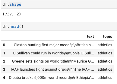
DataFrameを用いるサンプルコードのデータはTextheroのサンプル内にあるBBCのレポートを使う。

import texthero as hero
import pandas as pd

df = pd.read_csv(
   "https://github.com/jbesomi/texthero/raw/master/dataset/bbcsport.csv"
)

f:id:chito_ng:20210606114949p:plain

前処理

自然言語に対して諸々おこなうにあたって、タグの削除や名寄せのための処理（空白の削除や大文字小文字の統一など）を行う必要がある。このライブラリを使わない場合は正規表現でがんばったりする必要があるが（英語であれば）ある程度の処理用メソッドが用意されている。

texthero.org

ただし、現状では日本語未対応なので日本語に対してこのあたりの処理は以下の記事のように相変わらず自分でやる必要がある。

qiita.com

前処理メソッド

様々な前処理用のメソッドがあるので、例示する。なお、例示をしやすいのでpandas.seriesで示しているが通常通りDFに対しても可能。

# データ読み込み
row_text = "    Hi! I've started kàgglé,   and I'm enjoying."
s = pd.Series(row_text)
# =>     Hi! I've started kàgglé,   and I'm enjoying.

# スペースの削除
hero.remove_whitespace(s)
# =>Hi! I've started kàgglé, and I'm enjoying.

# ダイアクリティカルマーク（発音区別符号。àやéなど）の削除
hero.remove_diacritics(s) 
# =>    Hi! I've started kaggle,   and I'm enjoying.

 # 小文字への統一
hero.lowercase(s)
# =>   hi! i've started kàgglé,   and i'm enjoying.

# ストップワードの削除
from texthero import stopwords

default_stopwords = stopwords.DEFAULT # プリセット
custom_stopwords = default_stopwords.union(set(["Hi"]))


hero.remove_stopwords(s, custom_stopwords) 

# =>    I started kàgglé    I enjoying

clean

hero.cleanでは上述含む、一般的によくされるような前処理は一括でおこなってくれる。
具体的には、デフォルトで以下のメソッドがまとめて処理される。

fillna(s) Replace not assigned values with empty spaces.
lowercase(s) Lowercase all text.
remove_digits() Remove all blocks of digits.
remove_punctuation() Remove all string.punctuation (!"#$%&'()*+,-./:;<=>?@[]^_`{|}~).
remove_diacritics() Remove all accents from strings.
remove_stopwords() Remove all stop words.
remove_whitespace() Remove all white space between words.

# cleanで小文字処理やいらんスペースなどよしなに処理
df['clean_text'] = hero.clean(df['text'])

f:id:chito_ng:20210606120719p:plain

なお、Textheroではpipe処理をすると可読性よく処理できる。

df['clean_text'] = df['text'].pipe(hero.clean) # pipeでの書き方

# 以下と等価
# df['clean_text'] = hero.clean(df['text'])

また、デフォルトと異なる処理をしたい場合はpipeline引数に処理メソッドをリストで渡す。

from texthero import preprocessing

custom_pipeline = [preprocessing.fillna,
                   preprocessing.lowercase,
                   preprocessing.remove_whitespace]

df['clean_text'] = hero.clean(df['text'], pipeline=custom_pipeline)

# 等価
# df['clean_text'] = df['clean_text'].pipe(hero.clean, custom_pipeline)

解析

named_entitiesで各単語が人物名なのか、地名なのかなど解析してラベリングをしてくれる（正直性能が微妙な気もする)。
こちらも日本語未対応。

具体的なラベルは以下

PERSON: People, including fictional.
NORP: Nationalities or religious or political groups.
FAC: Buildings, airports, highways, bridges, etc.
ORG : Companies, agencies, institutions, etc.
GPE: Countries, cities, states.
LOC: Non-GPE locations, mountain ranges, bodies of water.
PRODUCT: Objects, vehicles, foods, etc. (Not services.)
EVENT: Named hurricanes, battles, wars, sports events, etc.
WORK_OF_ART: Titles of books, songs, etc.
LAW: Named documents made into laws.
LANGUAGE: Any named language.
DATE: Absolute or relative dates or periods.
TIME: Times smaller than a day.
PERCENT: Percentage, including ”%“.
MONEY: Monetary values, including unit.
QUANTITY: Measurements, as of weight or distance.
ORDINAL: “first”, “second”, etc.
CARDINAL: Numerals that do not fall under another type.

s = pd.Series("Yesterday I was in NY with Bill de Blasio")
hero.named_entities(s)[0]

# [('Yesterday', 'DATE', 0, 9),
# ('NY', 'GPE', 19, 21),
#  ('Bill de Blasio', 'PERSON', 27, 41)]

s = pd.Series("Crawford lived in KOBE 10 years ago with Tom")
hero.named_entities(s)[0]

# [('Crawford', 'ORG', 0, 8),
# ('KOBE', 'GPE', 18, 22),
# ('10 years ago', 'DATE', 23, 35),
#  ('Tom', 'PERSON', 41, 44)]

ベクトル変換

おそらく使用のメインになりそうなベクトル変換。現状用意されているのは以下。

DBSCAN
k-menas
MEAN SHIFT
NMF
PCA
tf(TERM FREQUENCY)
tf-idf
t-SNE

texthero.org

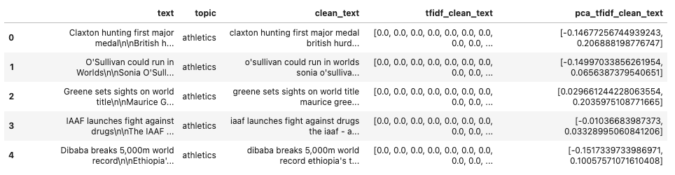
以下のサンプルはtf-idfとPCAを別カラムとして作成している。なお、次元数は各メソッドのデフォルトを使用。

custom_pipeline = [preprocessing.fillna,
                   preprocessing.lowercase,
                   preprocessing.remove_whitespace]

df['clean_text'] = df['clean_text'].pipe(hero.clean, pipeline=custom_pipeline))) # 前処理
df['tfidf_clean_text'] = hero.tfidf(df['clean_text']) # tf-idfでベクトル化
df['pca_tfidf_clean_text'] = hero.pca(df['tfidf_clean_text']) # PCAで2次元に写像

なお、それぞれ列を作らなくてもいい場合は以下のようにpipeを使った方が可読性が高い。

custom_pipeline = [preprocessing.fillna,
                   preprocessing.lowercase,
                   preprocessing.remove_whitespace]

df['pca'] = (
            df['text']
            .pipe(hero.clean, pipeline=custom_pipeline)) # 前処理
            .pipe(hero.tfidf)# tf-idfでベクトル化
            .pipe(hero.pca) # PCAで2次元に写像
   )

f:id:chito_ng:20210606124115p:plain

可視化

ワードクラウドと単語の頻度ランキング、散布図が作成できる。散布図はわざわざtexthero経由でやらなくてもいい気もするが、ベクトル化した値は[x, y, z, ...]のように文字列で入るのでseabornなどを使う際は正規表現で抜いてきたり、多次元の場合は列数が増えたりして面倒だが、texthero経由だとそのまま扱うことができる。

texthero.org

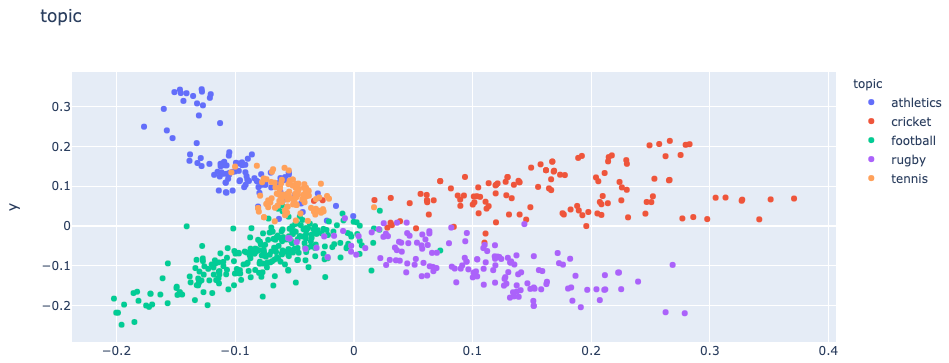
散布図

hero.scatterplot(df, 'pca_tfidf_clean_text', color='topic', title='topic')

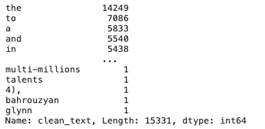
f:id:chito_ng:20210606124347p:plain

ワードランキング

hero.top_words(df['clean_text'])

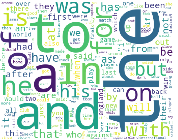
f:id:chito_ng:20210606124454p:plain

ワードクラウド

日本語の場合などフォント指定したい場合は、fontpathでダウンロードしたフォントを指定する

hero.visualization.wordcloud(df['clean_text'], 
                            colormap='viridis', 
                             width=500,
                             height=400, 
                             background_color='White')

# 日本語の場合はオプションに font_path='fonts/NotoSansCJKJP/NotoSansCJKjp-Regular.otf' などとする

f:id:chito_ng:20210606124830p:plain