ggplot2覚書① 棒グラフ

今までなんとなくでggplot2を使っていたので「Rグラフィッククックブック」を使って、ちゃんと覚えてなかったりする部分のメモ

Rグラフィックスクックブック ―ggplot2によるグラフ作成のレシピ集

なお、「Rグラフィッククックブック」はggplot2のバージョンが古いのでオプションのデフォルトが変わっていたりの関係で一部動かないので注意。

基本的にはhelp呼び出して読めばなんとなくはわかるけど、ggplot2のチートシートも参照すると色々便利。

棒グラフ

geom_barのデフォルトstatはcount

xのグループに従ったyの数値を棒グラフで取りたい。

library(ggplot2)
library(gcookbook)

ggplot(cabbage_exp, aes(x=Date, y=Weight, fill=Cultivar)) +
  geom_bar(position="dodge")
# =>エラー: stat_count() must not be used with a y aesthetic.

geom_barのstatはデフォルトではcountになる。countでは指定したxの個数を数えるためyは必要ないのでエラーになる。

geom_bar(mapping = NULL, data = NULL, stat = "count",
  position = "stack", ..., width = NULL, binwidth = NULL,
  na.rm = FALSE, show.legend = NA, inherit.aes = TRUE)

そのため、明示的にstat = "identity"を指定する必要がある。

ggplot(cabbage_exp, aes(x=Date, y=Weight, fill=Cultivar)) +
  geom_bar(position="dodge", stat = "identity")

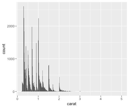
ヒストグラム

stat = "count"では連続値の場合は各値に対してcountされる。

ggplot(diamonds, aes(x=carat)) + 
  geom_bar(stat="count")

ヒストグラムを書きたい場合、stat = "bin"にする。

ggplot(diamonds, aes(x=carat)) + 
  geom_bar(stat="bin")

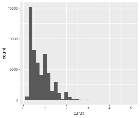
ちなみに、ヒストグラム用のgeom_histgramでも書ける。

ggplot(diamonds, aes(x=carat)) + 
  geom_histogram()

色の指定

棒グラフの内部の色はfillに指定したグループ毎に自動で分けられる。また、枠線はcolorで指定ができる。
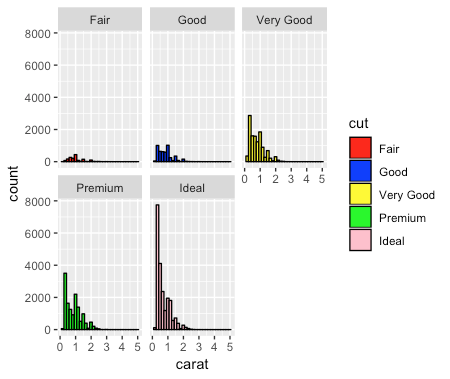
fillを任意の色で指定したい場合はscale_fill_manualを用いる

ggplot(diamonds, aes(x=carat, fill = cut)) + 
  geom_histogram(color = "black") +
  scale_fill_manual(values=c("red", "blue", "yellow", "green", "pink")) +
  facet_wrap(~cut)

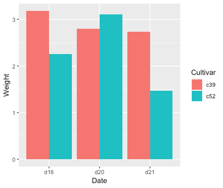
棒の位置

積み上げか並列か

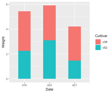
同じx軸内でfillなど指定で別グループがある場合、デフォルトではposition = "stack"なので、積み上げになる。

ggplot(cabbage_exp, aes(x=Date, y=Weight, fill=Cultivar)) + 
  geom_bar(stat="identity", width=0.5)

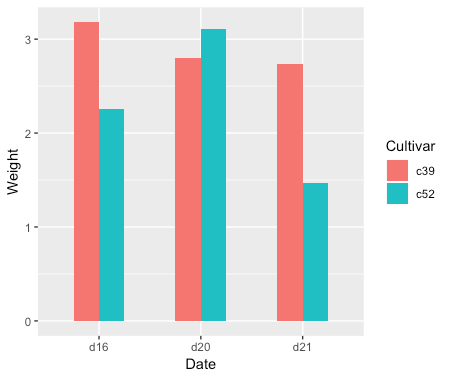
position = "dodge"で並列になる。

ggplot(cabbage_exp, aes(x=Date, y=Weight, fill=Cultivar)) + 
  geom_bar(stat="identity", width=0.5, position = "dodge")

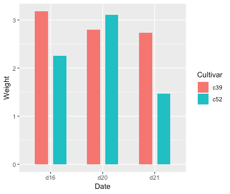
また、positionにposition_dodgeを指定することでdodgeの位置指定もまとめておこなえる。 このとき、widthより大きな値を指定すると棒グラフの位置が離れる(width, position_dodgeのデフォルトは0.9)。

ggplot(cabbage_exp, aes(x=Date, y=Weight, fill=Cultivar)) + 
  geom_bar(stat="identity", width=0.5, position=position_dodge(0.7))

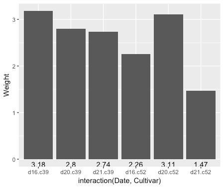
数値ラベルをつける

棒グラフの大きさを表す値を数値でつけるには、geom_textを使う。

ggplot(cabbage_exp, aes(x=interaction(Date, Cultivar), y=Weight)) +
  geom_bar(stat="identity") + 
  geom_text(aes(label=Weight, y = Weight), vjust=1.5, colour="white")

yを指定することでy軸の値に則って指定することができる。上記コードではマッピングされたy(Weight = 棒グラフの上点)を0としてvjustで位置を指定している。今回は明示的に示したが、デフォルトはこのようになっている。aes外で指定すると空間自体に位置していができる。

ggplot(cabbage_exp, aes(x=interaction(Date, Cultivar), y=Weight)) +
  geom_bar(stat="identity") + 
  geom_text(aes(label=Weight), vjust=1.5, colour="black", y = 0)